In this example we will have a simple column chart that will exclude a column of data from the visible chart, but not from our Excel sheet. It’s very easy to do and involves simply unchecking a check box in the Select Data Source dialog box.

In this example we have three columns of data over a series of a few years. We have three types of groceries. In the chart, there is also a linear trend line for the meat category. We have a chart title and an axis title for each axis.

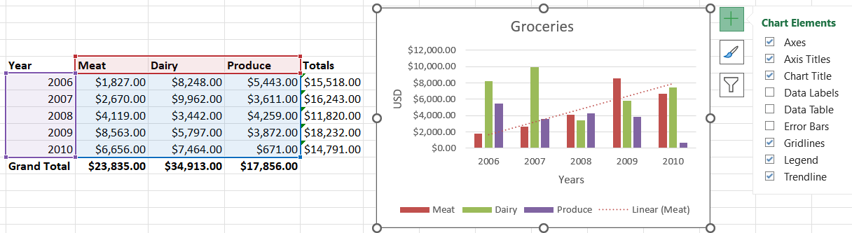
Now we want to hide the produce in the chart and only show the meat and dairy. You don’t need to create a second chart if you don’t want to. We can just de-select the category we want to hide. How do we do this?

Select the chart and click on the Chart Design Menu. Click Select Data. In the Legend Entries Series section of the Select Data Source dialog box, uncheck Produce.

The chart changes as shown below.