Do you have an Excel workbook (file) that has multiple worksheets of data that you need to combine into one sheet and create a pivot table so that you can analyze the combined data? Suppose the worksheets we have are representing different geographic locations of a retail chain. Each worksheet has very similar column headings but they are not in the same order. They are however named the same, which is important. Another example is where each sheet represents a different time period, such as a month. You have 12 sheets for the year and you want to combine them into a year.

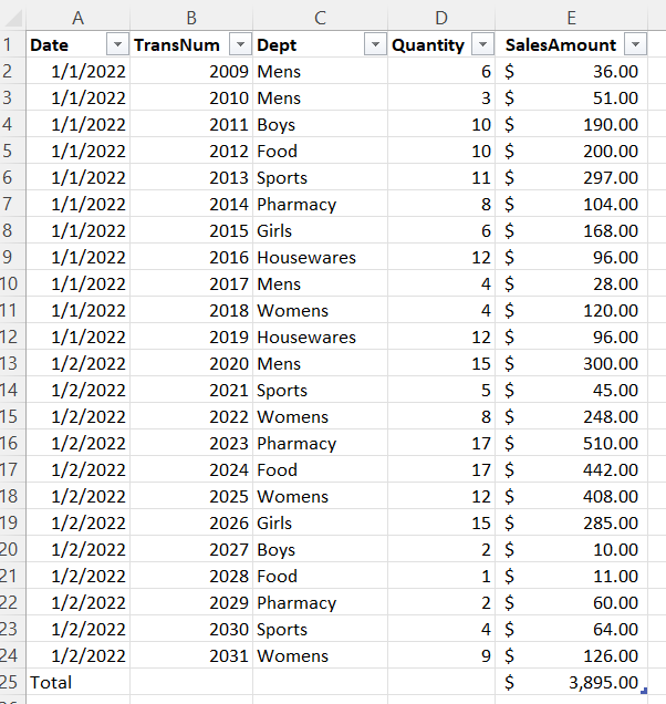
Let’s take a look at the data we have to start with. This is in an Excel file I have called TwoStores.xlsx. I have two worksheets, one is called Store1 and the other is called Store2. I have converted the data into tables (use shortcut Ctrl+T) and named the tables tblStore1 and tblStore2. I have also made that the data types in each table make sense. The Transaction date is formatted as a Short Date, the quantity and Sales Amounts are formatted as Numbers and Accounting, and the rest are General. These types can be found on the Home tab. I have also added a total row by checking the Total Row box in the Table Design tab. Below are two screenshots of tblStore1 and tblStore2.

Power Query

Before getting into Power Query, I will check to see that there are no Total Rows in any of the tables. If there are, I will remove them. If I don’t do that, Power Query will try to import that row as part of the data, which I don’t want.

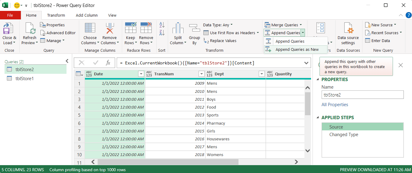
Go to the Store2 worksheet. Click inside the table. Click on the Data tab. Click From Table/Range in the Get and Transform group. The Power Query Editor opens.

When I get into Power Query, I will find that I will want to change the Date type to be a Date and not include the Time because I don’t need the time. I won’t be analyzing Time because there is no Time data in the original tables anyway. You can click Replace Current in the dialog box. I may find that I want to change the SalesAmount to a currency number instead of a whole number since it is currency.

After any transformation, I need to just create a connection. To do that, in the Power Query Editor, I go to Close & Load, Close & Load To… and select Only Create Connection. Repeat this process for the other worksheet.

Double-click one of your Queries shown in the Queries and Connections pane to open Power Query. Next we need to Append these two queries together, as shown on the below screenshot.

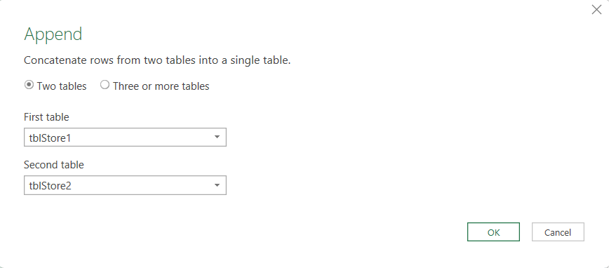
Choose both stores as shown below.

Rename it from Append1 to something more descriptive like AllStores or perhaps BothStores. Do that on the right-hand side, as shown in the below screenshot.

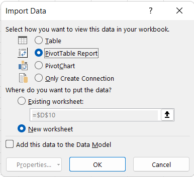
Close and Load, Clocse and Load To, Pivot Table Report.

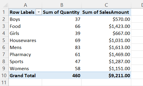
We now can set up our Pivot Table. I have dragged Dept to the Rows and Sum of Quantity and Sum of SalesAmount to the Values. Also I formatted the Sales Amount as a currency by clicking a data item, right-clicking the mouse and choosing Number Format, Currency.

Filter by Store

As it is now, we can’t filter by the store because we have merged the data. We could add a column to our original sheet or we could add it to Power Query. Which one is better? I suggest adding it to Power Query. We don’t want to change our original data sheets for the stores in any way because we might need to do this over and over again and it would be much easier to use Power Query to do this.

Click on the Store1 or Store2 worksheet and double-click on a Store in the Queries & Connection pane to open Power Query. In the Power Query Editor, click the Add Column tab (menu) at the top. Add a Custom Column.

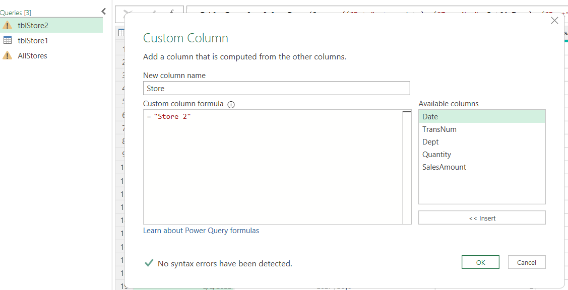
The column is added on the right side at the end. Change the data type to a text column. We will do it for Store 1 also. At the left, double-click All Store to see if it was appended properly. If not, in the last step, be sure that you named the added columns the same name. Perhaps you called it Store, as I did. Click Home. Close and Load.

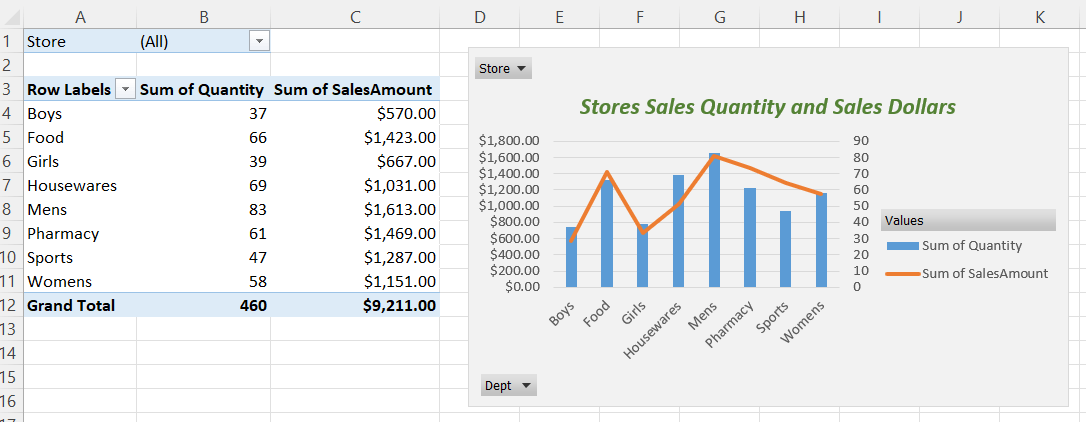
Double-click All Stores to get to the Pivot Table. Now we need to Refresh. Click inside the Pivot table, right-click and choose Refresh. Add Store to the Filter part of the Pivot Table. I have added a combo chart with a bit of formatting.

Learning with YouTube

If you would like to watch a YouTube on this topic, try Create a Pivot Table from Multiple Sheets in Excel | Comprehensive Tutorial! by Leila Gharani. Have a look at time 1:28 to 6:44. In the video, we are interested in method one. In Power Query, we need to create connections and then append queries. In the Power Query Editor, go to the File menu, Combine, Append Queries, AppendQueries as New.