Relationships Between Variables
Up to this point we’ve looked at univariate measures, those with one variable. We’ve looked at a single variable measures already (univariate measures) and talked about central tendency, asymmetry, and variability. Now we’ll look at multivariate measures. This post is about covariance and the linear correlation coefficient. So let’s examine the relationship between variables.
The Number of Variables
Data in statistics is sometimes classified according to how many variables are in a particular study. For example, “height” might be one variable and “weight” might be another variable. Depending on the number of variables being looked at, the data might be univariate, it might be bivariate, or even multivariate.
Bivariate analysis studies two variables. For example, if you are studying ice cream sales and the temperature for the day. In bivariate analysis, you will be looking at two columns of data in a table. Bivariate analysis might involve scatter plots, regression analysis, and correlation coefficients.
Here are a few things that seem intuitive, but are they true? Generally, the more square feet a house is the higher the price. On average, the taller a person is, the more they weigh. The newer a car is, the higher the price/value. The rarer the gemstone is, the higher the price/value. The hotter the weather, the more ice cream you will sell, and so on.
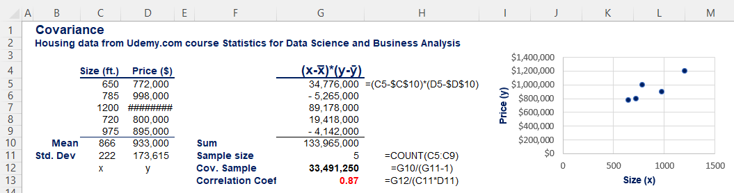
In our exploratory data analysis (EDA) we could use a scatter plot to have a look at some of our data points. We could use formulas. Once again, there is a sample and a population formula. Suppose we just have 2 columns of data in Excel, one for square feet and one for price.

The above formula is for sample data. If we had the population, it would be N, not n-1 in the denominator.

Values always range from -1 for a perfectly inverse, or negative, relationship to 1 for a perfectly positive correlation. Values at, or close to, zero indicate no linear relationship or a very weak correlation. The range is from -1 to +1. No correlation would be 0.
We got a correlation coefficient of 0.87. That is strong. Assessments of correlation strength based on the correlation coefficient value vary by application. In physics and chemistry, a correlation coefficient should be lower than -0.9 or higher than 0.9 for the correlation to be considered meaningful, while in social sciences the threshold could be as high as -0.5 and as low as 0.5. If we got one as the result, we’d have a perfect positive correlation, where the entire variability of one variable is explained by the other variable.
Remember, correlation does not imply causation. Two completely separate things could be correlated statistically, but in no way does one cause the other.
The correlation between two variables x and y is the same as the correlation between y and x. The formula is completely symmetrical with respect to both variables. Therefore, the correlation of price and size is the same as the one of size and price. This leads us to causality. It is very important for any analyst or researcher to understand the direction of causal relationships. In the housing business, size causes the price, and not vice versa. If price goes up, the size doesn’t change.
If you are working in Python, you can create a correlation heatmap with the seaborn package.