What if we had two populations to consider? So far we’ve been looking at single populations.
In some cases, the samples that we have taken from the two populations will be dependent on each other and in others they will be independent. Dependent samples can occur in several situations. First, when we are researching the same subject over time. Examples are weight loss and blood samples. Essentially, we are looking at the same person before and after. If we’re looking at husbands and wives, we’re looking at dependent samples.
Consider another example from the Udemy course Statistics for Data Science and Business Analysis. We can have the same people but in samples relating to different things. So instead of a before-and-after situation, we are looking at cause and effect. For example, when applying to university in the US, you sit the SAT, and based on it you either get admitted or you don’t. The applicant is the same person. However, the samples are different – one relates to the SAT, and the other – to the admittance outcome.
| Dependent | Independent |
|---|---|
|
|
Dependent Samples – People Before and After
Here’s an example from the Udemy.com course Statistics for Data Science and Business Analysis where we consider the effectiveness of a magnesium supplement. We’ll look at the before and after blood tests. Healthy people have between 1.7 and 2.2 mg per deciliter (dL). We would have our list of people in one column, the before column, the after column, and the new difference column. We could just use the Student’s T statistic and calculate it just like we had a single population.
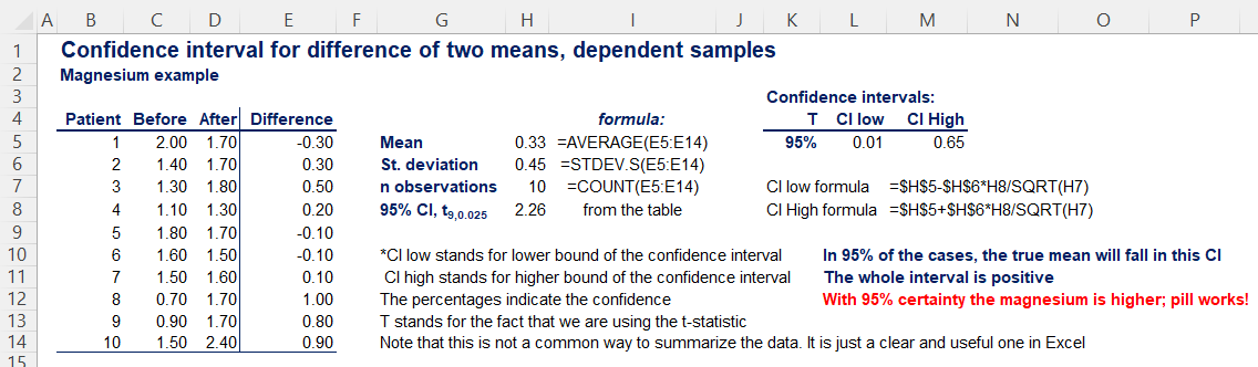
We are working with differences between the before measurement and the after measurement. The formula looks a bit different. We have a low sample size so we’ll use the Student’s t statistic. Here is what the formula looks like.

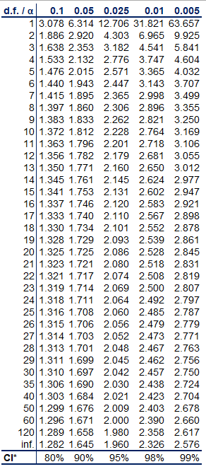
We need to use the Students T table. We have 10 samples so that’s 9 degrees of freedom. We want a 95% confidence interval. We can go to the bottom of the chart to find 95%. Alternatively, at the top of the chart, we’ll look for (1 – 95%)/2, which is 0.025. When we find the intersection of 9 and 95%, we get 2.262.