The Student’s T-distribution is one of the most important breakthroughs in statistics, as it allowed inference through small samples with an unknown population variance.

This post describes how to construct a confidence interval for a small sample size. Note that large samples use Z-scores and small samples use T-scores. How small is small. Generally about 30 or fewer is considered a small sample size.

Confidence intervals for small sample sizes only deal with population means, and not population proportions. The statistical reason for this distinction is somewhat technical.

Although large samples give more precise estimates than small samples, collecting a small sample is usually less expensive and time-consuming than collecting a large sample. Sometimes all we’ve got to work with is a small sample.

History

William Sealy Gosset (1876 – 1937) was an English statistician who worked for the brewery of Guinness. He developed different methods for the selection of the best-yielding varieties of barley. He was trying to develop a way to extract small samples but still come up with meaningful predictions. He published several papers that are still relevant today. However, due to the Guinness company policy, he was not allowed to sign the papers in his own name. Therefore, all of his work was under the pen name: Student.

This distribution looks like the normal distribution, but it is more dispersed and has fatter tails. just like the z-statistic is related to the standard normal distribution, the t-statistic is related to the Student’s t distribution.

The bigger the sample, the closer we get to the population’s numbers. In fact, a common rule of thumb is that for a sample containing more than 50 observations, we use the z-table instead of the t-table.

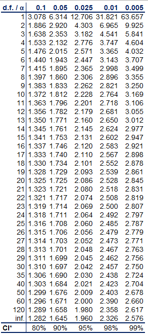
With the t statistics, we have something new: degrees of freedom. If we have 12 observations, we have 11 degrees of freedom, and with 20 observations we have 19 degrees of freedom. We can use a table to find the t statistic. To use the table, we need two things: the degrees of freedom and alpha. Alpha can be calculated from the desired confidence interval. For 95%, alpha will be 5%. For 99%, the alpha is 1%.

When we do not know the population variance, we can still make predictions, but they will be less accurate. The proper statistic for estimating the confidence interval when the population variance is unknown is the t-statistic and not the z-statistic.

Here above is the formula.

Let’s work on an example. Recall that the standard error is the standard deviation divided by the square root of the sample size.

• The sample size is 9 (n)
• Sample Mean is 92533 (s)
• Standard Deviation of sample is 13932
• Standard Error is 4644
• We use the t statistic (population variance unknown)
• We have 8 degrees of freedom (9-1)

When we use the table shown below for 8 degrees of freedom and a confidence interval of 99%, we get a t statistic of 3.335. Let’s round that to 3.36. After we plug in the values into the formula, we can say that with 99% certainty, the salaries of the population will be between $76,930 and $108,137.

A common rule of thumb is that if we have more than 50 observations in our sample, we can use the t table instead of the z table because the numbers are almost the same anyway.

Learn from other Websites

Here’s an article from Scribbr.com called T-Distribution | What It Is and How To Use It (With Examples).