We have a series of posts that introduces the reader to decision trees. It begins with the post called Decision Trees Modelling Introduction. I recommend reading that before jumping into the code shown here.

This is a simple example of creating a simple decision tree in Python. In this example I am using Jupyter Notebook. The data is only seven rows long and is from the Coursera course called The Nuts and Bolts of Machine Learning. There is a module in that course that is called Tree-based modelling.

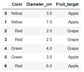
Here is the original data shown in a DataFrame in Jupyter Notebook.

Below is a cell of Markdown, not code. The following cell is also Markdown.

# Decision Tree - Apples and Grapes
This is from Google's Advanced Data Analytics Course at Coursera. See the module The Nuts and Bolts of Machine Learning. There are five modules in that course. Module four is called Tree-based Modelling. 

## Modeling objective
The modeling objective is to build and test a decision tree model that uses data to predict the type of fruit. It will either be an apple or gtrape. We will build a decision tree that will take new data and based on the predictor variables, it will estimate the type of fruit.

Import libraries.

import numpy as np
import pandas as pd
import matplotlib.pyplot as plt

from sklearn.tree import DecisionTreeClassifier

# This function displays the splits of the tree
from sklearn.tree import plot_tree

Normally we would split the data, but to keep things really simple we will not. If we wanted to split the data we would import it from sklearn.model_selection import train_test_split. Next we read in the data file. You can create your own data file.

# manually create the dataset instead of importing it.
data = {'Color': ['Yellow','Yellow','Red','Red','Green','Green','Red'],
       'Diameter_cm': [3.5,7,2,2.5,4,3,6],
       'Fruit_target': ['Apple','Apple','Grape','Grape','Grape','Apple','Apple']}
df_original = pd.DataFrame(data)
df_original

Check the class balance. We know there are 4 apples and 3 grapes in the dataset.

# Check class balance
df_original['Fruit_target'].value_counts()

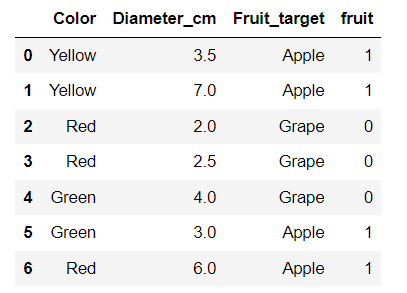
Encode the fruit column

# create a custom function
def fruit_encode(fruit):
    if fruit == 'Apple':
        x = 1
    else:
        x = 0
    return x

# make a copy to preserve the original data for a future reference.
df_0 = df_original.copy()

# create a new column called fruit that's an encoded Fruit_target
df_0['fruit'] = df_0['Fruit_target'].apply(fruit_encode)
df_0

# Create a new df that drops Fruit_target column because we have fruit
df_1 = df_0.drop(['Fruit_target'], axis=1)
df_1

# Dummy encode categorical variables and create a new DataFrame
df_2 = pd.get_dummies(df_1, drop_first=False)
df_2

# Define the y (target) variable
y = df_2['fruit']

# Define the X (predictor) variables
X = df_2.copy()
X = X.drop('fruit', axis=1)

Here is where we would normally split the dataset into training data and test data. I am not going to do that here, just to keep things simple.

# Instantiate the model
decision_tree = DecisionTreeClassifier(random_state=0)

# Fit the model to training data
decision_tree.fit(X, y)

# Plot the tree
plt.figure(figsize=(15,12))

plot_tree(decision_tree, max_depth=4, fontsize=12, feature_names=['Diameter_cm', 'Color_Green', 'Color_Red', 'Color_Yellow'], 
          class_names=['grape', 'apple'], filled=True);
plt.show()

Here is what the plot looks like in Jupyter Notebook. Please click on it to enlarge it.

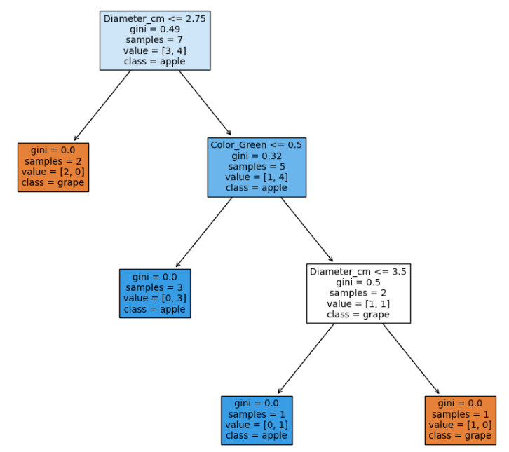
The next post in this series of posts discusses the plotted tree. It’s called Plot Tree Interpretation.