Many of the transformations in Power Query are fairly easy to grasp but other ones, such as Pivotting and Unpivotting are not as intuitive. This post offers two examples of unpivoting. The first one is a simple example of pivoting. The second one from Maven Analytics is more interesting.

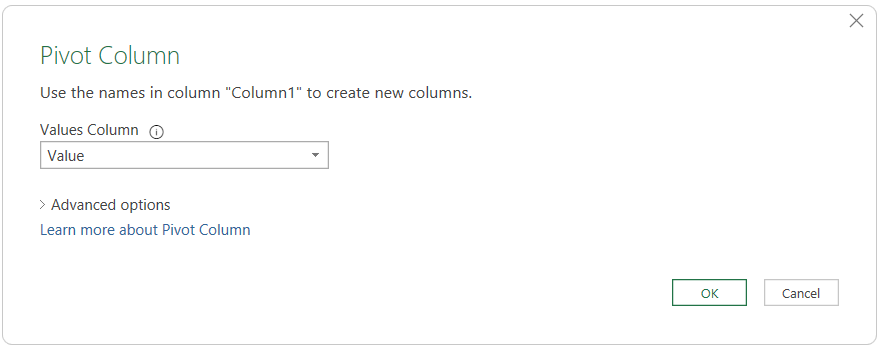
To pivot is to turn distinct rows into columns.

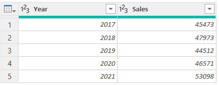
After we pivot on the Sales column we get the following.

Notice that in this second example we have duplicate years. We have two rows of yesr 2017.

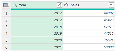
When we transpose this we find that the year 2017’s sales value is aggregated into a sum.

Maven’s Pivot Unpivot Example

Chris Dutton from Maven has an example of using Excel’s Power Query to transform a small data set to get it in a proper form. It’s from a course at Udemy called Microsoft Excel: Business Intelligence w/ Power Query & DAX and it’s video number 23.

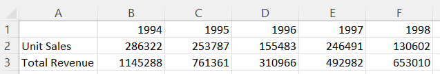
Let’s bring it into Power Query. I have created a range and given it the name RangeData. It is A1 to F3. In the Data tab (menu), choose From Table/Range. Once inside Power Query you can promote the headers.

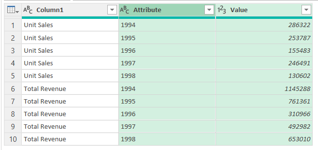
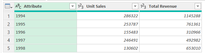
Now we want a column for Unit Sales and a column for Total Revenue with the years in a column at the left.

Here below is our result.

Are you working in Python and pandas? Have a look at the melt() function. In pandas, have a look at .T. This is transpose.