Combining or appending data from multiple sheets is a common task in Excel. We’ll show you how you can stack multiple data sets vertically with a single formula. We’ll use Microsoft Excel’s new VSTACK function. It is dynamic.
Let’s look at an example. Suppose you have a series of worksheets similar to the one shown below. You need to combine them into one. Perhaps you have several geographic locations that each send their daily sales to the head office for combining into sales for the day for the whole company.
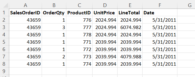
In our example we have three worksheets: Sales1, Sales2 and Sales3. Here is our worksheet called Combine, after writing our VSTACK function. When writing your formula, please make sure that the number of rows specified is large enough. Here I have only use F15, for 15 rows of data. Be sure to use a number large enough to exceed the largest number of rows in any of your worksheets. We will remove those zeros in the next example.

To remove those zeros we just need to add the FILTER function to our formula. Below is the next example, I have decided to change the 15 to a 20 for the number of rows, just to be safer.

In the next example I am sorting the results by the ProductId, ascending. The formula requires the column number. ProdiuctId is the third column, so we have the number 3 in the SORT forrmula. The 1 means ascending. Negaitive one is descending.

Next we’ll sort first by ProductId ascending, then by LineTotal descending. In the formula we use curly braces and put the column numbers in the first brace and the sort orders in the second brace.

Dynamic
If there are any updates and changes to any of the worksheets, they will be reflected in the VSTACK function, automatically. You can also add more worksheets to the workbook and VSTACK will be updated provided that the range of worksheets is inclusive of the new worksheet. Also, we would want to do some column formatting on the date and currency columns.