What is a slicer? A slicer is a visual representation of a filter. They are available in Excel 2010 onwards. When you have rows and columns of data you may find that you need to filter that data to see only certain rows. When you create a Table or a Pivot Table in Excel, you automatically get the filter buttons appear at the top of each row. In this example, I created a table with Ctrl+T. Users can click on that “down arrow” and choose which rows they want to see. The others are still there, but they are hidden.

In my example I have a table from Itzik Ben-Gan’s database. It is the Orders table.

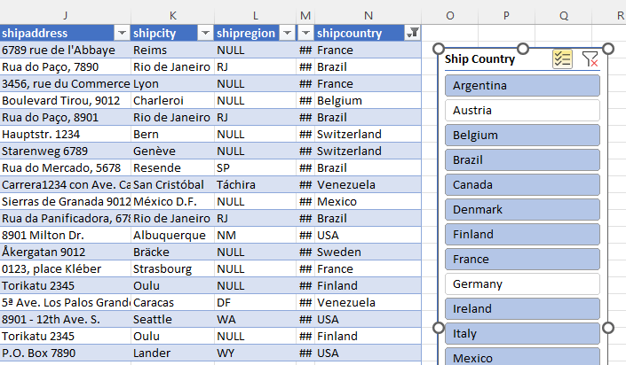
I have inserted the Slicer and made a couple of adjustments. To insert a slicer, first be sure that you have selected somewhere inside your table. One way to insert a slicer is to go to the Insert tab (menu) and clcik on Slicer. You will get a popup dialog that lists all of the column headings. Go ahead and check as many as you need.

I clicked on the Multi-Select button at the top of the slicer. It has check marks and lines icons. In this way I can now select more than one from the list. I clicked on a few countries to deselect them. Slicers are objects and they can be easily moved around on the worksheet. One slicer can actually filter more that one table at the same time.

Multiple Slicers

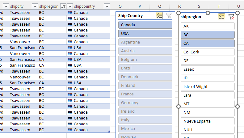
You can have many sliders for one table. Notice that if I choose BC and CA in the Region, the Country shows Canada and USA and the other countries are grayed out because BC and CA are within those two countries and do not apply to any other country.

Formatting Slicers

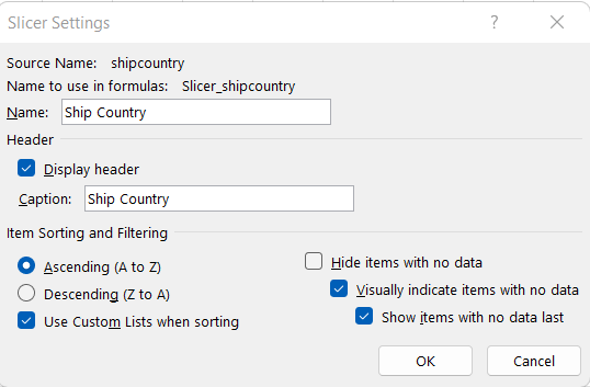
After right-clicking on the edge of the slicer and choosing Slicer Settins, I set the Name and the Caption to Ship Country from shipcountry. Below is the slicer settings window.

Select a slicer. You should see the Slicer tab at the top. It might say Slicer Tools instead. You can see that I have changed the color of the slicer. I gave it a better caption. I gave the slicer two columns so it would fit better on the screen. We have Align tools so we can place the slicers neatly. When moving a slicer, the Alt key will snap the slicer and the Shift key will keep in it the same horizontal or vertical plane, depending on how you move it.

A slicer can actually be on a different worksheet than the table is on. You could use Copy and Paste to achieve this.

Suppose, for the sake of the users of the slicer, you didn’t want those pull handles to be activated when the user clicks on the slicer. To prevent this, select the slicer. Right-click. Go to Size and Properties… In the Format Slicer pane, under Position and Layout, select Disable resizing and moving. This is a great feature when you are building dashboards.

To connect one slicer to more than one table or pivot table, right-click the slicer and go to Report Connections. Choose your tables. The following screenshot is from OnlineTrainingHub.com’s Excel file example from the video mentioned below in the YouTube section of this post.

Learn with YouTube

You could have a look at Mynda Treacy’s video from MyOnlineTrainingHub.com that’s called Excel Slicers, Inside Out – includes workbook with step by step instructions.

Here’s a video called Excel Slicers – The Cool Way to Filter Data! It’s by Sele Training. It’s 10 minutes long.