This post is about filtering in Excel. For information on the FILTER function have a look at our post called Excel Filter Function.

You can filter various ways. You can filter by numbers or text. You can even filter by the cell’s background color.

When you copy a filtered range and then paste that range in another location you only get the rows that were copied. This can be handy. You can filter your data down to less and less data without deleting any of your original data. In this way you can verify your filtered data to ensure the filter was done correctly.

Learn with YouTube

Here’s a 16 minute video by Kevin Statvert that’s called How to Filter in Excel. He uses a range of data that has filter “drop-downs”. Here’s a video by Leila Gharani that’s under 11 minutes long, that’s called Excel Filter Basics (for quick data analysis).

Advanced Learn with YouTube

Here’s an interesting video from Leila Gharani that has a “trick” I didn’t know until now. The video is called SURPRISING Advanced Filter TRICK in Excel (You’ve Never Heard Of!). Ok so spoiler alert here!. The trick is in the Advanced filter. You filter your range and copy it to another location (another sheet for example) and at the same time only copy over the columns you want. Of course you can use multiple criteria as well. In this example, the data is a range, not a table.

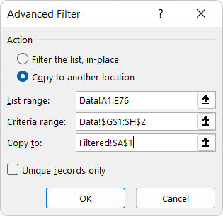
Using the sample data in Excel in the Home tab’s Analyze Data button, I set up the Data tab;s Advanced Filter dialog box as follows. I have an original Excel sheet called Data and a results sheet called Filtered. When you are ready to create the filter, start in the sheet that the result set will go, which in this case is the Filtered sheet. I put my cursor in cell A1, clicked the Data tab and then Advanced Filter. Before doing all of this I added the data to the sheet and added some criteria, as you can see.

Below is the screenshot of part of the first sheet.

Below is a screenshot of the Advanced Filter dialog box.