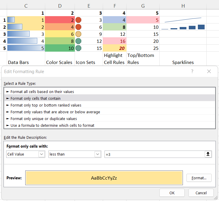
Conditional formatting is a spreadsheet tool that changes how cells appear when values meet specific conditions. Here we’ll just look at a quick conditional format example with Microsoft Excel. We have a multiplication table. This shows a few examples of Conditional formatting, which is found in the Home menu. I’ve also added a sparkline example for comparison, in column H in the screenshot below. Sparklines are not conditional formatting, but they do offer an additional way to display data without the real estate overhead of a chart.
Please click on the screenshot below to see an example of a number of different formatting rules. For the data bars in column C, I first selected the data in column C from C2 to C6 and clicked Conditional Formatting in the Home menu. Click the screenshot below to enlarge it.

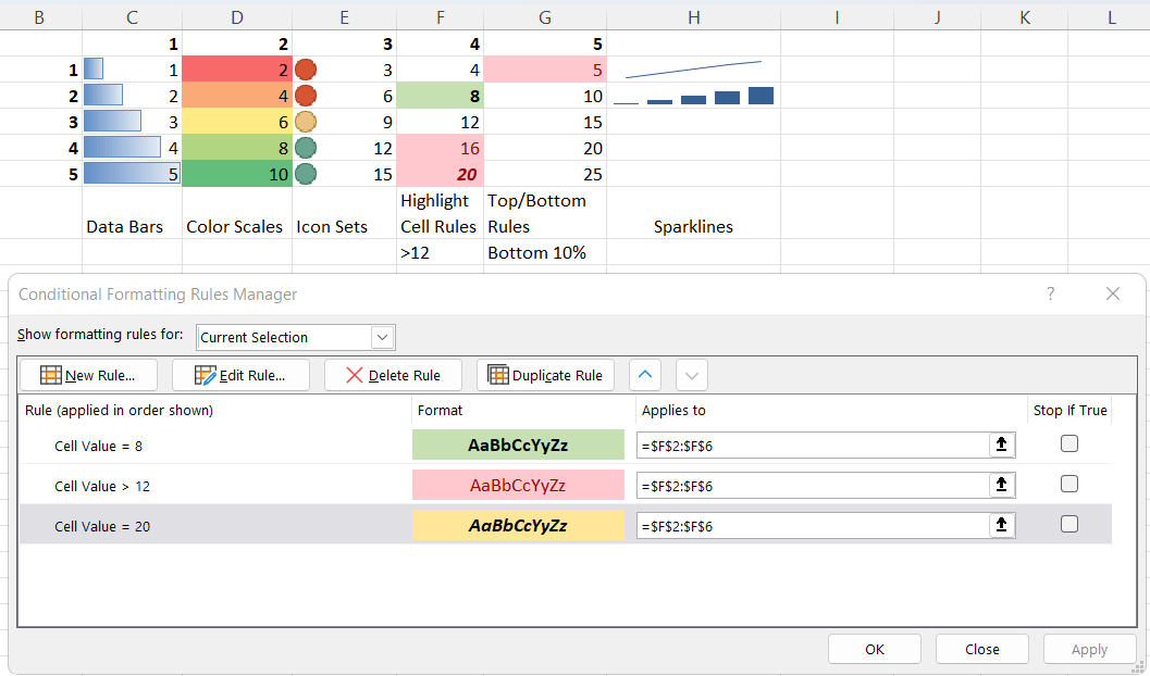
The most complex part of this is the three rules I have used for column F. I used the Manage Rules dialog to add rules. You can see the three rules in the screenshot also notice that in cell F6, the value of 20 is true for two of the three rules. First, it does equal 20 so it is formatted italic with a yellow background. However, 20 is also greater than 12, so it should be formatted with a green background. You can see that the italic and yellow color won the battle because it is higher on the list. If you were to select the “yellow” rule and move it to the bottom of the list with the down arrow button, and click Apply, you will find that the cell F6 will now have a red background, but it will retian an italic font.
When there is a rule conflict, the top rule wins. In this example, the conflict was with the background color, not whether it was italic or not.
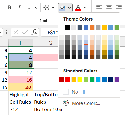
Formatting the background color of cells F2 and F3 with a blue background color does not change the background color of cell F3 because that cell meets a condition in our conditional formatting. What does this mean? This means that conditional formatting overrides the set formatting of a cell, as long as the condition is met. This is what you would expect. Please click on the graphic below. Observe the small red box around one of the blue colors. Also notice that the two cells are selected.
We can have more than one conditional format applies to the same set of cells, as we can see in column C in the screenshot below. Here I am showing what I did to add the second condition with the yellow background.