Use VLOOKUP when you need to find things in a table or a range by row. For example, look up a price of an automotive part by the part number, or find an employee name based on their employee ID. VLOOKUP stands for Vertical Lookup. As the name implies, this function is used to look up a value in one column and return a value in another column, on the same row. Before using VLOOKUP, ensure that your data is clean and in the proper format. By format I mean that numbers are formatted as numbers and not text. Dates should probably be in the date format and not a string format. To do that you might use the VALUE function. Also, by format I mean that there are not any extra spaces in the data. You could use TRIM for this. Also, watch out for duplicates.

The value that you are searching for has to be in a range that is the left-most column and the value that you want returned has to be in an adjacent column.

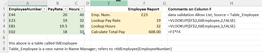
=VLOOKUP(What you want to look up, where you want to look for it, the column number in the range containing the value to return, return an Approximate or Exact match – indicated as 1/TRUE, or 0/FALSE).

VLOOKUP (lookup_value, table_array, col_index_num, [range_lookup])

Takeaways

• it only returns the first match it finds
• it can only look to the right for the value, so you may need to copy and paste a column
• be careful with your absolute references when copying
• may need to adjust the formula when inserting new columns
• consider protecting the sheet
• TRUE is for approximate matches and FALSE is for exact matches

With XLOOKUP, you can look in one column for a search term and return a result from the same row in another column, regardless of which side the return column is on.

Learning with YouTube

Here is a YouTube tutorial called VLOOKUP in Excel | Tutorial for Beginners that’s by Kevin Stratvert.

Here is another YouTube tutorial on VLOOKUP. It’s by Leila Gharani and it’s called Excel VLOOKUP: Basics of VLOOKUP and HLOOKUP explained with examples.