The normal distribution is a continuous probability distribution that is symmetrical on both sides of the mean and bell-shaped. The normal distribution is often called the bell curve because its graph has the shape of a bell with a peak at the center and two downward-sloping sides. It is also known as the Gaussian distribution after the German mathematician Carl Gauss who first described the formula for the distribution. It has no skew.

In contrast, discrete probability distributions where the outcomes of experiments are represented by countable whole numbers. For example, rolling a die can result in a two or three, but not a decimal value such as 2.852.

The normal distribution is the most common probability distribution in statistics because so many different kinds of data sets display a bell-shaped curve.

The standard normal distribution has a mean of zero and a standard deviation of one.

The above formula means Normal distribution (~ means distribution) with a mean and variance. Sorry for the look of the tilde. The tilde (~) should have spaces around it and be in the middle instead of at the top.

Distribution

In statistics, when we use the term distribution, we usually mean a probability distribution. As examples, there are the Normal distribution, the Binomial distribution, and the Uniform distribution. A distribution is a function that shows the possible values for a variable and how often they occur. This might be a good time to review probability and the histogram.

Consider rolling one fair die. You have an equal chance of getting either a 1, 2, 3, 4, 5, or 6. discrete uniform distribution. All outcomes have an equal chance of occurring. This is a discrete distribution. In the real world, we are often working with continuous distributions. In health care we may be working with heights or weights of people or animals.

In statistics, we focus on the Normal distribution and the Student’s T distributions rather than the Uniform, Binomial, or Poisson distributions. The Normal distribution is also called the Gaussian distribution, but many people call it the Bell Curve as it is shaped like a bell. It is symmetrical and its mean median and mode are equal. It has no skew. N stands for Normal. N ~ (μ, σ^2)

Regarding the normal distribution, a lower standard deviation results in a lower dispersion, so more data is in the middle and it has thinner tails. A higher standard deviation will cause the graph to flatten out with fewer points in the middle and more to the end, or “fatter tails”.

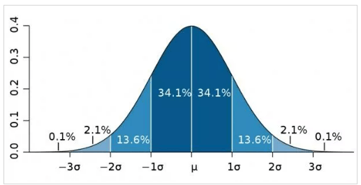
Below is a diagram of the standard normal distribution.

Standardization

The next post in this series is on standardization. This will come up again when we get to hypothesis testing.