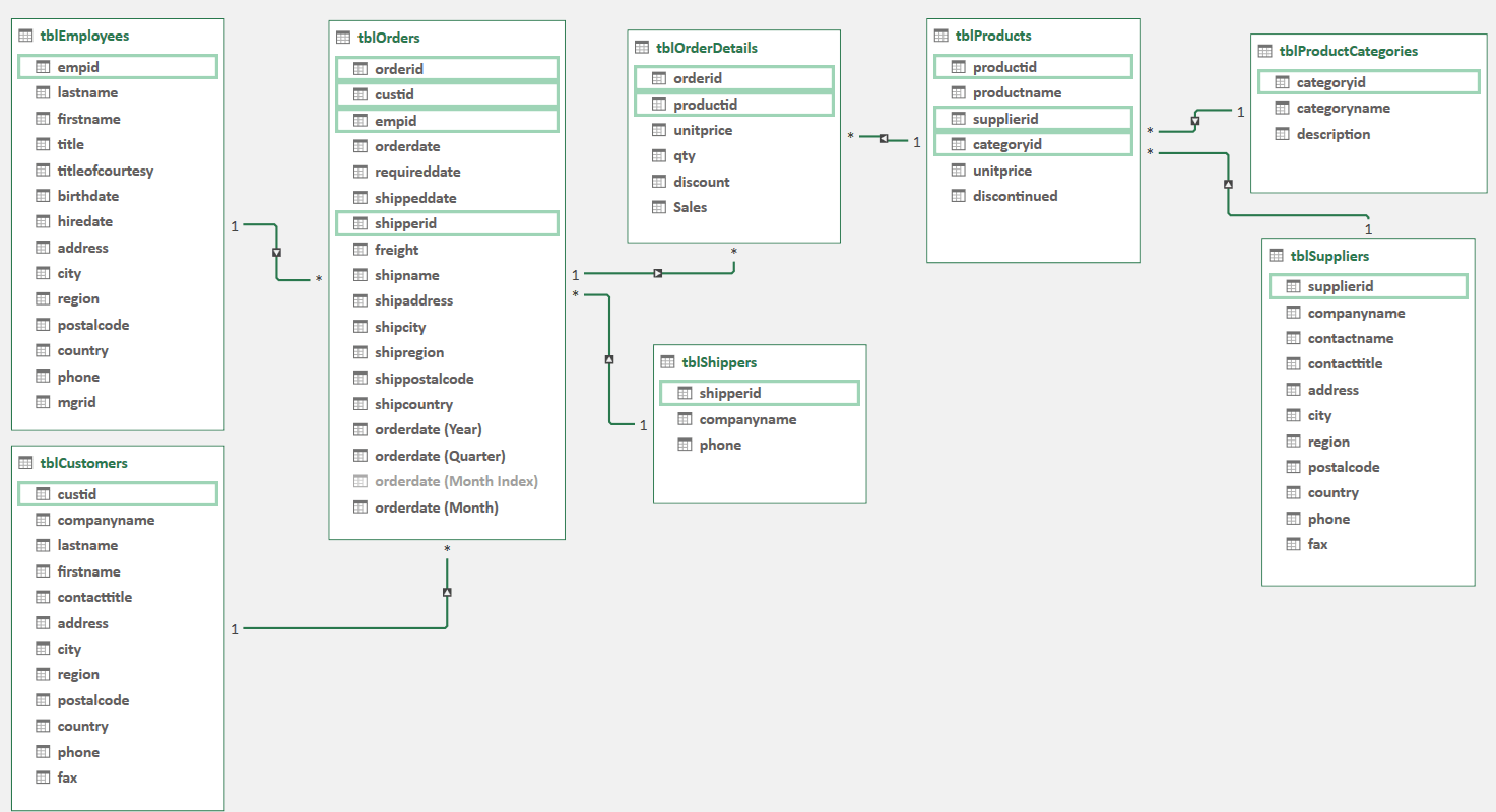
As a more complex and realistic example, let’s look at the database that Itzik Ben-Gan used in his book T-SQL Querying, or at least most of the tables in the database. Check out our other post on this database called Itzik Ben Gan’s SQL Database.

Below is a screenshot of Itzik’s data model in Excel’s Power Pivot. Click on it to enlarge it. Once it’s in the data model of Excel, you can create pivot tables to analyze the data and create charts.

Getting the Data

At the book’s website there is a way to download the SQL script that if run in SSMS (or another suitable program) you can get the table and the data into a SQL Server database. There are a few ways to get the data into Excel. I just selected the results of a SELECT statemewnt, copied the data with headers and pasted it into a blank Excel sheet. I did that for each table. Then I use Ctrl+T to make tables and named the tables with a ‘tbl” prefix. I saved and named the Excel workbook ItzikRawTables.xlxs.

Power Query

Next, I created a new Excel file and made connections to each of the sheets. How do you do that? In your new Excel file, click on the Data tab. Now we need to get the data. Click on Get Data, From File, From Excel Workbook. Navigate to the Excel file with the raw data, which in my case was called ItzikRawTables.xlxs. Click Import. Click on the first table, which in my case was called tblCustomers. Click Transform Data button. This is important because we need to use Power Pivot to do a small amount of necessary cleaning. In this post, I won’t go through every transformation, but suffice it to say that you need to check your data types and be sure to replace NULL with null. NULL in the data is a text string, and we need to ensure that in Excel it truly becomes null, not a text string. When you are satisfied we’ve made the necessary transitions and data cleaning, click Close & Load, Close & Load To…, and in the dialog box click Only Create Connection and Add this data to the data Model.

I created a calculated column called Sales in the order details table. Here is the formula: =tblOrderDetails[unitprice]*tblOrderDetails[qty]*(1-tblOrderDetails[discount]).

Now you can create a Pivot table and a Pivot chart, like the one below. We are bringing in data from two joined tables here. We are getting data from the tblOrderDetails and from tblProductCategories.

Here is what the pivot looks like. It’s quite simple.

Structured Query Language (SQL)

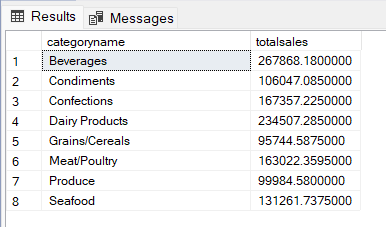
What would the SQL be that generates that table of data? The name of the tables are a bit different in Itzik’s actual database, but you can see that we required two LEFT JOINs to make it work. The LEFT JOIN keyword returns all records from the left table, and the matching records from the right table.

SELECT Production.Categories.categoryname,
       SUM([Sales].[OrderDetails].[unitprice]*[Sales].[OrderDetails].[qty]*(1-[Sales].[OrderDetails].[discount])) As "totalsales"
  FROM [TSQLV3].[Sales].[OrderDetails]
  LEFT OUTER JOIN Production.Products ON [Sales].[OrderDetails].productid = Production.Products.productid
  LEFT OUTER JOIN Production.Categories ON Production.Products.categoryid = Production.Categories.categoryid
  GROUP BY Production.Categories.categoryname
  ORDER BY categoryname

Here is what it looks like in SSMS.

Switching the order, we can sort by “totalsales” descending (DESC) with the following change to the SQL: ORDER BY totalsales DESC. This will match our Excel example.